The WRAPROWS function in Google Sheets is a powerful tool that facilitates the restructuring of data into a more manageable format. By allowing users to take a range of cells in either rows or columns and arrange them into a new array with a specified number of elements per row, this function promotes better organization and readability of data sets.

Syntax

WRAPROWS(range, wrap_count, [pad_with]) 

• range: It asks which range of cells to wrap.
• wrap_count: Asks what is the maximum amount of cells that each row should have. The value will be rounded to the nearest whole number.
• [pad_with]: If you have extra cells in the range, you can fill it with this value. By default, its filled with the #N/A.

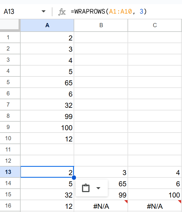
Example #1

=WRAPROWS(A1:A10, 3)

This function will take the range A1 through A10 and reorganize it into rows with 3 elements each. The resulting array will look something like this: you see that #N/A are filled in the last 2 cells of the range as extra cells.

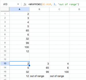
Example #2

=WRAPROWS(A1:A10, 3, "out of range")

Like in the previous function it shows the data in 3 rows, but this time also with “out of range” message in the extra cells.

Error handling

• REF!: This error occurs if the specified range includes cells that are outside the valid range of the sheet.
• VALUE!: This error indicates that an invalid argument was passed, typically a non-numeric value for num_rows.
• N/A: This error means that the function could not find applicable data in the chosen range.

Conclusion

The WRAPROWS function provides users of Google Sheets with a convenient means of transforming data into structured arrays. By specifying a maximum number of elements per row, this function not only enhances the organization of data but also improves overall readability. Embracing WRAPROWS can greatly facilitate data management tasks, making it an essential tool for anyone looking to optimize their workflow in Google Sheets.