Are vector-databases the new craze?

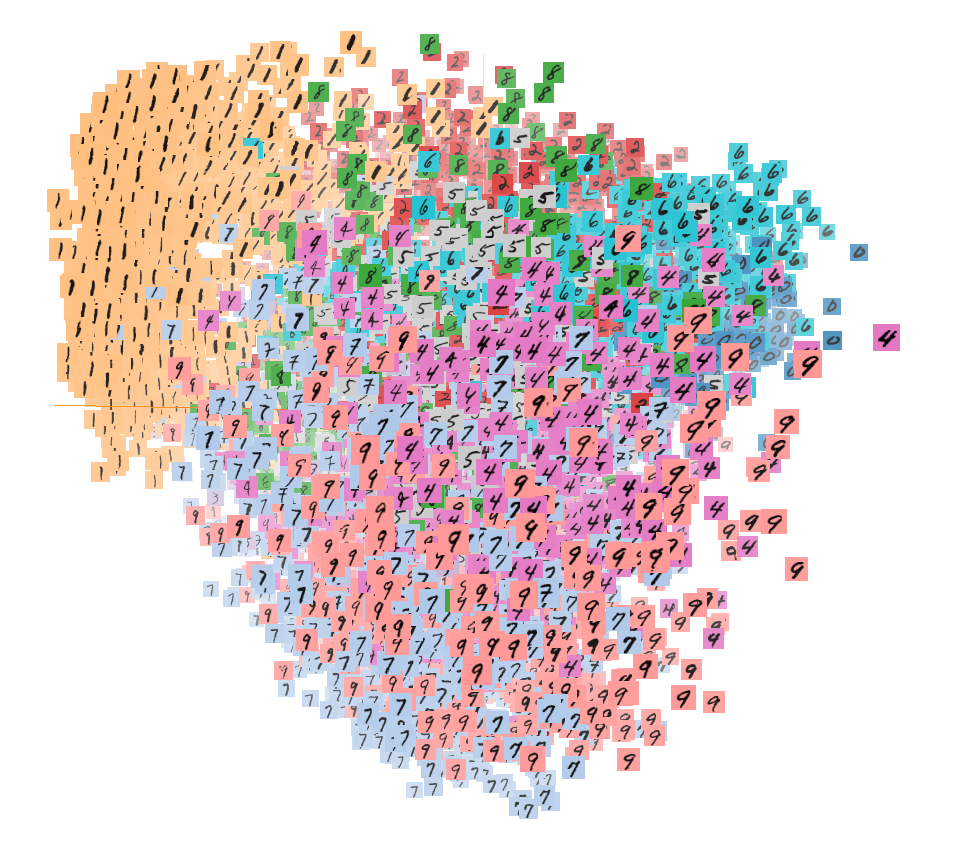
Unlike traditional databases that use a row-column-architecture, vector-databases use vectors to represent their data. For reference a vector is a 1-dimensional array of numbers like [0.64, 0.32, 0.97]. This means that there isn’t a set grid where the vectors can be placed while still being able to do classical operations. All these vectors get stored in an embedding which is like a room with many dimensions.

Each value in a vector corresponds with a dimension in the embedding. This way like classical databases you can display similarities and differences by making vectors have similar values in one dimension but differentiate in another dimension. If you “look” at an embedding, you will see that similar objects group together as if they were pulled by a magnet.

Why are vector-databases superior?

Thanks to the way that every vector is saved, many different tasks become much more efficient than in other databases. Making a query is very easy as similar vectors already are “next” to each other. Before each vector gets added they get “indexed” which maps them to a data-structure and makes searching faster.

When a query gets requested, you can use an algorithm like cosine-similarity to calculate the nearest vectors and output them. Speaking of queries, filters can also be added by doing pre- or postfiltering which filters the queried results or queries the filtered data. Compared to other database-structures querying shows a faster runtime which makes it useful when dealing with unstructured data like websites or posts in social-media platforms like Twitter, Facebook or Instagram.

Vector-databases at code-level

Let’s look at how we can get the cosine similarity of 2 vectors using Python. We’ll use numpy to get the dot-multiplication of both vectors and then normalize them. You get the similarity by dividing the dot-product with the product of both normalized vectors. Here is the code to do this:

import numpy as np

def cosine_similarity(vector1, vector2):
    dot_product = np.dot(vector1, vector2)
    norm_vector1 = np.linalg.norm(vector1)
    norm_vector2 = np.linalg.norm(vector2)
    similarity = dot_product / (norm_vector1 * norm_vector2)
    return similarity

# Example 
vector1 = [0.867, 0.446, 0.236]
vector2 = [0.164, 0.648, 0.948]
similarity = cosine_similarity(vector1, vector2)

#Output: 0.5628393553089471

As you can see we got an output from around 0.56 meaning they aren’t that similar (1 = 100% match; 0 = 0% match).

Search query

Still this isn’t as efficient if you are dealing with many vectors. Let’s look at another algorithm.

# Using KNN algorithm
from sklearn.neighbors import NearestNeighbors
import numpy as np

def find_k_nearest_neighbors(X, query_vector, k):
    # Create an instance of NearestNeighbors
    nbrs = NearestNeighbors(n_neighbors=k, algorithm='kd_tree').fit(X)

    # Find k-nearest neighbors
    distances, indices = nbrs.kneighbors(query_vector)

    # Return the k-nearest neighbors
    return distances, indices


# Example usage
# Generate a random dataset
X = np.random.rand(100, 10)

# Query vector
query_vector = np.random.rand(1, 10)

# Find 5-nearest neighbors
k = 5
distances, indices = find_k_nearest_neighbors(X, query_vector, k)

In this code we are generating 100 random vectors each having 10 dimensions. Then we will be doing a search query with a vector also having 10 dimensions. To accomplish this, we will be using the KNN algorithm. If you want to learn more about this algorithm, you can read about it here. Be warned as it this enters a field of advanced mathematics. This is the output:

print("K-nearest neighbors:")
for i in range(k):
    print("Neighbor:", i+1)
    print("Distance:", distances[0][i])
    print("Index:", indices[0][i])
    print("Vector:", X[indices[0][i]])
    print()

# Output:
query_vector = [[0.1113187  0.75351452 0.9374165  0.76445506 0.68385283 0.72236542
  0.70277158 0.77592412 0.28326503 0.07586657]]
k = 5

# K-nearest neighbors:
# Neighbor: 1
# Distance: 0.6807253770735626
# Index: 32
# Vector: [0.04212379 0.25497311 0.98374969 0.50389832 0.79652829 0.65142171
# 0.53587406 0.75926397 0.03879164 0.2613137]

# Neighbor: 2
# Distance: 0.8165762180854882
# Index: 8
# Vector: [0.1940449  0.97680781 0.6981634  0.26523264 0.73049437 0.64620033
# 0.52062487 0.44178118 0.6714971  0.06594126]

# Neighbor: 3
# Distance: 0.825618290080734
# Index: 52
# Vector: [0.43931076 0.35308087 0.7583844  0.99293407 0.23197408 0.78826507
# 0.57181333 0.55572981 0.07441403 0.1839082 ]

# Neighbor: 4
# Distance: 0.9181803452355117
# Index: 31
# Vector: [0.84097593 0.94434338 0.66560885 0.55546493 0.78160776 0.61385801
# 0.70407179 0.41658848 0.33249874 0.01417456]

# Neighbor: 5
# Distance: 0.9434755476918664
# Index: 97
# Vector: [0.15430003 0.00618319 0.49802488 0.79061649 0.41424987 0.73832103
# 0.55142175 0.64870304 0.22348331 0.21883166]

As we can see the 5-nearest neighbors are listed from most similar to least similar.

Conclusion

With more data being added to the internet than ever old and slow databases can’t keep up that fast. That’s why new and efficient ways have to be found to deal with everything. Vector-databases are a brilliant example for this. Even though they aren’t quite new recently they have gone in the spotlight. Many companies and projects with vector databases have been funded in the past few months like Pinecone. Also, Microsoft announced that they will start developing vector search capability in Azure Cognitive Search, which is a big step forward for a better way to store and search data.

Interested in databases? Find more articles here!