GETPIVOTDATA is one of my favorite functions in Excel when it comes to retrieving and aggregating data. Its similar to SUMIFS and CUBEVALUE, but it always references a pivot table.

What is the GETPIVOTDATA function?

The GETPIVOTDATA function is a built-in function in Excel that allows you to retrieve data from a pivot table based on specific criteria. You can use this function to extract values, subtotals, or grand totals from a pivot table, and to create formulas that reference pivot table data dynamically.

The syntax of the GETPIVOTDATA function is:

=GETPIVOTDATA(data_field, pivot_table, [field1, item1, field2, item2, ...])

The parameters of the GETPIVOTDATA function are:

– data_field: The name of the value field in the pivot table that you want to get data from. This must be enclosed in quotation marks.

– pivot_table: A reference to any cell or range of cells within the pivot table.

– field1, item1, field2, item2, …: Optional pairs of field names and items that specify the criteria for the data you want to retrieve. Each field name must be enclosed in quotation marks, and each item must match the exact text or value in the pivot table.

How to use the GETPIVOTDATA function?

To use the GETPIVOTDATA function, you need to have an existing pivot table in your worksheet or in another worksheet in your Excel file. You can then enter the function in any cell outside the pivot table, and specify the data_field, pivot_table, and any field-item pairs that match your criteria.

Examples

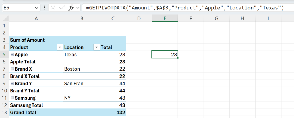
The easiest way to generate GETPIVOTDATA is to start typing “=” in a cell outside of a pivot table and then point click with the mouse somewhere inside a pivot table. This will result in the formula being generated automatically as in example below.

To disable generating GETPIVOTDATA, which sometimes can be annoying, you can easily insert a “Generate Getpivotdata” checkbox on top of your ribbon:

Referencing Cells

You can also use cell references instead of hard-coded values for the field-item pairs, as long as they match the text or value in the pivot table. For example, if you have the product name in cell A10 and the region name in cell B10, you can use the following formula:

=GETPIVOTDATA(“Sales”,B4,”Product”,A10,”Region”,B10)

This will return the same result as the previous formula, but it will update automatically if you change the values in A10 or B10.

What are the benefits of using the GETPIVOTDATA function?

The GETPIVOTDATA function has several advantages over using a simple cell reference to get data from a pivot table. Some of the benefits are:

– Its easy to use and setup: just click-point at the pivot table and the function is generated.

– It can retrieve subtotals or grand totals from the pivot table easily and perform ratios calculations

– It can be combined with other functions or operators to perform calculations or comparisons on the pivot table data.

One known disadvantage of GETPIVOTDATA is that you always need to have your pivot table setup somewhere to get referenced and if you change its filters or fields, then the formula breaks.

You can read my further articles on using GETPIVOTDATA here: Excel CUBEVALUE vs SUMIFS & GETPIVOTDATA » Data Empower

If you would like to share an idea, leave a comments below!